In computer graphics, the terms parametric continuity (Ck) and geometric continuity (Gn) were introduced by Brian Barsky, to show that the smoothness of a curve can be measured either with respect to a particular parametrization or after allowing changes in the speed with which the parameter traces out the curve.123
Parametric continuity
Parametric continuity (Ck) is a concept applied to parametric curves, which describes the smoothness of the curve as a function of its parameter. A (parametric) curve is said to be of class Ck if the derivatives of up to order exist and are continuous on , where derivatives at the end-points and are taken to be one-sided derivatives (from the right at and from the left at ).
As a practical application of this concept, a curve describing the motion of an object with a parameter of time has C1 continuity when its velocity varies continuously, and C2 continuity when its acceleration varies continuously. For smoother motion, such as that of a camera's path while making a film, higher orders of parametric continuity may be required.
Order of parametric continuity

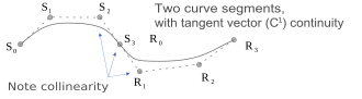
The various orders of parametric continuity can be described as follows:4
- : zeroth derivative is continuous (curves are continuous)
- : zeroth and first derivatives are continuous
- : zeroth, first and second derivatives are continuous
- : 0-th through -th derivatives are continuous
Geometric continuity
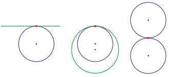

pencil of conic sections with G2-contact: p fix, variable
(: circle,: ellipse, : parabola, : hyperbola) source ↗
A curve or surface can be described as having continuity, with being an increasing measure of smoothness. Consider the segments on either side of a point on a curve:
- : The curves touch at the join point.
- : The curves also share a common tangent direction at the join point.
- : The curves also share a common center of curvature at the join point.
In general, continuity holds when the curves can be reparameterized so that they have parametric continuity.56 A reparametrization of the curve is geometrically identical to the original; only the parameter is affected.
Equivalently, two vector functions and such that have continuity at the point where they meet if they satisfy equations known as Beta-constraints. For example, the Beta-constraints for continuity are:
where , , and are arbitrary, but is constrained to be positive.5: 65 In the case , this reduces to and , for a scalar (i.e., the direction, but not necessarily the magnitude, of the two vectors is equal).
While it may be obvious that a curve would require continuity to appear smooth, for good aesthetics, such as those aspired to in architecture and sports car design, higher levels of geometric continuity are required. For example, class A surface requires or higher continuity to ensure smooth reflections in a car body.
A rounded rectangle (with ninety-degree circular arcs at the four corners) has continuity, but does not have continuity. The same is true for a rounded cube, with octants of a sphere at its corners and quarter-cylinders along its edges. If an editable curve with continuity is required, then cubic splines are typically chosen; these curves are frequently used in industrial design.
References
References
- Barsky, Brian A. (1981). The Beta-spline: A Local Representation Based on Shape Parameters and Fundamental Geometric Measures (Ph.D.). University of Utah, Salt Lake City, Utah.
- Brian A. Barsky (1988). Computer Graphics and Geometric Modeling Using Beta-splines. Springer-Verlag, Heidelberg. ISBN 978-3-642-72294-3.
- Richard H. Bartels; John C. Beatty; Brian A. Barsky (1987). An Introduction to Splines for Use in Computer Graphics and Geometric Modeling. Morgan Kaufmann. Chapter 13. Parametric vs. Geometric Continuity. ISBN 978-1-55860-400-1.
- van de Panne, Michiel (1996). "Parametric Curves". Fall 1996 Online Notes. University of Toronto, Canada. Archived from the original on 2020-11-26. Retrieved 2019-09-01.
- Barsky, Brian A.; DeRose, Tony D. (1989). "Geometric Continuity of Parametric Curves: Three Equivalent Characterizations". IEEE Computer Graphics and Applications. 9 (6): 60–68. doi:10.1109/38.41470. S2CID 17893586.
- Hartmann, Erich (2003). "Geometry and Algorithms for Computer Aided Design" (PDF). Technische Universität Darmstadt. p. 55. Archived (PDF) from the original on 2020-10-23. Retrieved 2019-08-31.