Superprocess

In probability theory, a superprocess is a measure-valued stochastic process that is usually constructed as a special limit of near-critical branching diffusions.

Informally, a superprocess can be seen as a branching process where each particle splits and dies at infinite rates, and evolves in a state space E according to a diffusion equation. We follow the rescaled population of particles, seen as a measure on E.

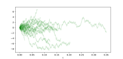
For any integer ${\displaystyle N\geq 1}$, consider a branching Brownian process ${\displaystyle Y^{N}(t,dx)}$ defined as follows:

• Start at ${\displaystyle t=0}$ with ${\displaystyle N}$ independent particles distributed according to a probability distribution ${\displaystyle \mu }$.
• Each particle independently move according to a Brownian motion.
• Each particle independently dies with rate ${\displaystyle N}$.
• When a particle dies, with probability ${\displaystyle 1/2}$ it gives birth to two offspring in the same location.

The notation ${\displaystyle Y^{N}(t,dx)}$ means should be interpreted as: at each time ${\displaystyle t}$, the number of particles in a set ${\displaystyle A\subset \mathbb {R} }$ is ${\displaystyle Y^{N}(t,A)}$. In other words, ${\displaystyle Y}$ is a measure-valued random process.¹

Now, define a rescaled process:

${\displaystyle X^{N}(t,dx):={\frac {1}{N}}Y^{N}(t,dx)}$

Then the finite-dimensional distributions of ${\displaystyle X^{N}}$ converge as ${\displaystyle N\to +\infty }$ to those of a measure-valued random process ${\displaystyle X(t,dx)}$, which is called a ${\displaystyle (\xi ,\phi )}$-superprocess,¹ with initial value ${\displaystyle X(0)=\mu }$, where ${\displaystyle \phi (z):={\frac {z^{2}}{2}}}$ and where ${\displaystyle \xi }$ is a Brownian motion (specifically, ${\displaystyle \xi =(\Omega ,{\mathcal {F}},{\mathcal {F}}_{t},\xi _{t},{\textbf {P}}_{x})}$ where ${\displaystyle (\Omega ,{\mathcal {F}})}$ is a measurable space, ${\displaystyle ({\mathcal {F}}_{t})_{t\geq 0}}$ is a filtration, and ${\displaystyle \xi _{t}}$ under ${\displaystyle {\textbf {P}}_{x}}$ has the law of a Brownian motion started at ${\displaystyle x}$).

As will be clarified in the next section, ${\displaystyle \phi }$ encodes an underlying branching mechanism, and ${\displaystyle \xi }$ encodes the motion of the particles. Here, since ${\displaystyle \xi }$ is a Brownian motion, the resulting object is known as a Super-brownian motion.¹

Our discrete branching system ${\displaystyle Y^{N}(t,dx)}$ can be much more sophisticated, leading to a variety of superprocesses:

• Instead of ${\displaystyle \mathbb {R} }$, the state space can now be any Lusin space ${\displaystyle E}$.
• The underlying motion of the particles can now be given by ${\displaystyle \xi =(\Omega ,{\mathcal {F}},{\mathcal {F}}_{t},\xi _{t},{\textbf {P}}_{x})}$, where ${\displaystyle \xi _{t}}$ is a càdlàg Markov process (see,¹ Chapter 4, for details).
• A particle dies at rate ${\displaystyle \gamma _{N}}$
• When a particle dies at time ${\displaystyle t}$, located in ${\displaystyle \xi _{t}}$, it gives birth to a random number of offspring ${\displaystyle n_{t,\xi _{t}}}$. These offspring start to move from ${\displaystyle \xi _{t}}$. We require that the law of ${\displaystyle n_{t,x}}$ depends solely on ${\displaystyle x}$, and that all ${\displaystyle (n_{t,x})_{t,x}}$ are independent. Set ${\displaystyle p_{k}(x)=\mathbb {P} [n_{t,x}=k]}$ and define ${\displaystyle g}$ the associated probability-generating function:${\textstyle g(x,z):=\sum \limits _{k=0}^{\infty }p_{k}(x)z^{k}}$

Add the following requirement that the expected number of offspring is bounded:$${\displaystyle \sup \limits _{x\in E}\mathbb {E} [n_{t,x}]<+\infty }$$Define ${\displaystyle X^{N}(t,dx):={\frac {1}{N}}Y^{N}(t,dx)}$ as above, and define the following crucial function:$${\displaystyle \phi _{N}(x,z):=N\gamma _{N}\left[g_{N}{\Big (}x,1-{\frac {z}{N}}{\Big )}\,-\,{\Big (}1-{\frac {z}{N}}{\Big )}\right]}$$Add the requirement, for all ${\displaystyle a\geq 0}$, that ${\displaystyle \phi _{N}(x,z)}$ is Lipschitz continuous with respect to ${\displaystyle z}$ uniformly on ${\displaystyle E\times [0,a]}$, and that ${\displaystyle \phi _{N}}$ converges to some function ${\displaystyle \phi }$ as ${\displaystyle N\to +\infty }$ uniformly on ${\displaystyle E\times [0,a]}$.

Provided all of these conditions, the finite-dimensional distributions of ${\displaystyle X^{N}(t)}$ converge to those of a measure-valued random process ${\displaystyle X(t,dx)}$ which is called a ${\displaystyle (\xi ,\phi )}$-superprocess,¹ with initial value ${\displaystyle X(0)=\mu }$.

Provided ${\displaystyle \lim _{N\to +\infty }\gamma _{N}=+\infty }$, that is, the number of branching events becomes infinite, the requirement that ${\displaystyle \phi _{N}}$ converges implies that, taking a Taylor expansion of ${\displaystyle g_{N}}$, the expected number of offspring is close to 1, and therefore that the process is near-critical.

The branching particle system ${\displaystyle Y^{N}(t,dx)}$ can be further generalized as follows:

• The probability of death in the time interval ${\displaystyle [r,t)}$ of a particle following trajectory ${\displaystyle (\xi _{t})_{t\geq 0}}$ is ${\displaystyle \exp \left\{-\int _{r}^{t}\alpha _{N}(\xi _{s})K(ds)\right\}}$ where ${\displaystyle \alpha _{N}}$ is a positive measurable function and ${\displaystyle K}$ is a continuous functional of ${\displaystyle \xi }$ (see,¹ chapter 2, for details).
• When a particle following trajectory ${\displaystyle \xi }$ dies at time ${\displaystyle t}$, it gives birth to offspring according to a measure-valued probability kernel ${\displaystyle F_{N}(\xi _{t-},d\nu )}$. In other words, the offspring are not necessarily born on their parent's location. The number of offspring is given by ${\displaystyle \nu (1)}$. Assume that ${\displaystyle \sup \limits _{x\in E}\int \nu (1)F_{N}(x,d\nu )<+\infty }$.

Then, under suitable hypotheses, the finite-dimensional distributions of ${\displaystyle X^{N}(t)}$ converge to those of a measure-valued random process ${\displaystyle X(t,dx)}$ which is called a Dawson-Watanabe superprocess,¹ with initial value ${\displaystyle X(0)=\mu }$.

A superprocess has a number of properties. It is a Markov process, and its Markov kernel ${\displaystyle Q_{t}(\mu ,d\nu )}$ verifies the branching property:$${\displaystyle Q_{t}(\mu +\mu ',\cdot )=Q_{t}(\mu ,\cdot )*Q_{t}(\mu ',\cdot )}$$where ${\displaystyle *}$ is the convolution.A special class of superprocesses are ${\displaystyle (\alpha ,d,\beta )}$-superprocesses,² with ${\displaystyle \alpha \in (0,2],d\in \mathbb {N} ,\beta \in (0,1]}$. A ${\displaystyle (\alpha ,d,\beta )}$-superprocesses is defined on ${\displaystyle \mathbb {R} ^{d}}$. Its branching mechanism is defined by its factorial moment generating function (the definition of a branching mechanism varies slightly among authors, some¹ use the definition of ${\displaystyle \phi }$ in the previous section, others² use the factorial moment generating function):

${\displaystyle \Phi (s)={\frac {1}{1+\beta }}(1-s)^{1+\beta }+s}$

and the spatial motion of individual particles (noted ${\displaystyle \xi }$ in the previous section) is given by the ${\displaystyle \alpha }$-symmetric stable process with infinitesimal generator ${\displaystyle \Delta _{\alpha }}$.

The ${\displaystyle \alpha =2}$ case means ${\displaystyle \xi }$ is a standard Brownian motion and the ${\displaystyle (2,d,1)}$-superprocess is called the super-Brownian motion.

One of the most important properties of superprocesses is that they are intimately connected with certain nonlinear partial differential equations. The simplest such equation is ${\displaystyle \Delta u-u^{2}=0\ on\ \mathbb {R} ^{d}.}$ When the spatial motion (migration) is a diffusion process, one talks about a superdiffusion. The connection between superdiffusions and nonlinear PDE's is similar to the one between diffusions and linear PDE's.

• Eugene B. Dynkin (2004). Superdiffusions and positive solutions of nonlinear partial differential equations. Appendix A by J.-F. Le Gall and Appendix B by I. E. Verbitsky. University Lecture Series, 34. American Mathematical Society. ISBN 9780821836828.

References

- Li, Zenghu (2011), "Measure-Valued Branching Processes", in Li, Zenghu (ed.), Measure-Valued Branching Markov Processes, Probability and Its Applications, Berlin, Heidelberg: Springer, pp. 29–56, doi:10.1007/978-3-642-15004-3_2, ISBN 978-3-642-15004-3, retrieved 2022-12-20
- Etheridge, Alison (2000). An introduction to superprocesses. Providence, RI: American Mathematical Society. ISBN 0-8218-2706-5. OCLC 44270365.